Tutorial
Speech Corpus Tools is a system for going from a raw speech corpus to a data file (CSV) ready for further analysis (e.g. in R), which conceptually consists of a pipeline of four steps:
- Import the corpus into SCT
- Result: a structured database of linguistic objects (words, phones, discourses).
- Enrich the database
- Result: Further linguistic objects (utterances, syllables), and information about objects (e.g. speech rate, word frequencies).
- Query the database
- Result: A set of linguistic objects of interest (e.g. utterance-final words ending with a stop),
- Export the results
- Result: A CSV file containing information about the set of objects of interest
Ideally, the import and enrichment steps are only performed once for a given corpus. The typical use case of SCT is performing a query and export corresponding to some linguistic question(s) of interest.
This tutorial is structured as follows:
Installation: Install necessary software – Neo4j and SCT.
Librispeech database: Obtain a database for the Librispeech Corpus where the import and enrichment steps have been completed , either by using a premade version, or doing the import and enrichment steps yourself.
Installation
Installing Neo4j
SCT currently requires that Neo4j version 3.0 be installed locally and running. To install Neo4j, please use the following links:
Once downloaded, just run the installer and it’ll install the database software that SCT uses locally.
SCT currently requires you to change the configuration for Neo4j, by doing the following once, before running SCT:
- Open the Neo4j application/executable (Mac/Windows)
- Click on
Options ... - Click on the
Edit...button forDatabase configuration - Replace the text in the window that comes up with the following, then save the file:
#***************************************************************
# Server configuration
#***************************************************************

# This setting constrains all `LOAD CSV` import files to be under the `import` directory. Remove or uncomment it to
# allow files to be loaded from anywhere in filesystem; this introduces possible security problems. See the `LOAD CSV`
# section of the manual for details.
#dbms.directories.import=import

# Require (or disable the requirement of) auth to access Neo4j
dbms.security.auth_enabled=false

#
# Bolt connector
#
dbms.connector.bolt.type=BOLT
dbms.connector.bolt.enabled=true
dbms.connector.bolt.tls_level=OPTIONAL
# To have Bolt accept non-local connections, uncomment this line:
# dbms.connector.bolt.address=0.0.0.0:7687

#
# HTTP Connector
#
dbms.connector.http.type=HTTP
dbms.connector.http.enabled=true
#dbms.connector.http.encryption=NONE
# To have HTTP accept non-local connections, uncomment this line:
#dbms.connector.http.address=0.0.0.0:7474

#
# HTTPS Connector
#
# To enable HTTPS, uncomment these lines:
#dbms.connector.https.type=HTTP
#dbms.connector.https.enabled=true
#dbms.connector.https.encryption=TLS
#dbms.connector.https.address=localhost:7476

# Certificates directory
# dbms.directories.certificates=certificates

#*****************************************************************
# Administration client configuration
#*****************************************************************


# Comma separated list of JAX-RS packages containing JAX-RS resources, one
# package name for each mountpoint. The listed package names will be loaded
# under the mountpoints specified. Uncomment this line to mount the
# org.neo4j.examples.server.unmanaged.HelloWorldResource.java from
# neo4j-examples under /examples/unmanaged, resulting in a final URL of
# http://localhost:${default.http.port}/examples/unmanaged/helloworld/{nodeId}
#dbms.unmanaged_extension_classes=org.neo4j.examples.server.unmanaged=/examples/unmanaged

#*****************************************************************
# HTTP logging configuration
#*****************************************************************

# HTTP logging is disabled. HTTP logging can be enabled by setting this
# property to 'true'.
dbms.logs.http.enabled=false

# Logging policy file that governs how HTTP log output is presented and
# archived. Note: changing the rollover and retention policy is sensible, but
# changing the output format is less so, since it is configured to use the
# ubiquitous common log format
#org.neo4j.server.http.log.config=neo4j-http-logging.xml

# Enable this to be able to upgrade a store from an older version.
#dbms.allow_format_migration=true

# The amount of memory to use for mapping the store files, in bytes (or
# kilobytes with the 'k' suffix, megabytes with 'm' and gigabytes with 'g').
# If Neo4j is running on a dedicated server, then it is generally recommended
# to leave about 2-4 gigabytes for the operating system, give the JVM enough
# heap to hold all your transaction state and query context, and then leave the
# rest for the page cache.
# The default page cache memory assumes the machine is dedicated to running
# Neo4j, and is heuristically set to 50% of RAM minus the max Java heap size.
#dbms.memory.pagecache.size=10g

#*****************************************************************
# Miscellaneous configuration
#*****************************************************************

# Enable this to specify a parser other than the default one.
#cypher.default_language_version=3.0

# Determines if Cypher will allow using file URLs when loading data using
# `LOAD CSV`. Setting this value to `false` will cause Neo4j to fail `LOAD CSV`
# clauses that load data from the file system.
dbms.security.allow_csv_import_from_file_urls=true

# Retention policy for transaction logs needed to perform recovery and backups.
dbms.tx_log.rotation.retention_policy=false

# Enable a remote shell server which Neo4j Shell clients can log in to.
#dbms.shell.enabled=true
# The network interface IP the shell will listen on (use 0.0.0.0 for all interfaces).
#dbms.shell.host=127.0.0.1
# The port the shell will listen on, default is 1337.
#dbms.shell.port=1337

# Only allow read operations from this Neo4j instance. This mode still requires
# write access to the directory for lock purposes.
#dbms.read_only=false

# Comma separated list of JAX-RS packages containing JAX-RS resources, one
# package name for each mountpoint. The listed package names will be loaded
# under the mountpoints specified. Uncomment this line to mount the
# org.neo4j.examples.server.unmanaged.HelloWorldResource.java from
# neo4j-server-examples under /examples/unmanaged, resulting in a final URL of
# http://localhost:7474/examples/unmanaged/helloworld/{nodeId}
#dbms.unmanaged_extension_classes=org.neo4j.examples.server.unmanaged=/examples/unmanaged
Installing SCT
Once Neo4j is set up as above, the latest version of SCT can be downloaded from the SCT releases page. As of 12 July 2016, the most current release is v0.5.
Windows
- Download the zip archive for Windows
- Extract the folder
- Double click on the executable to run SCT.
Mac
- Download the DMG file.
- Double-click on the DMG file.
- Drag the sct icon to your Applications folder.
- Double click on the SCT application to run.
LibriSpeech database
The examples in this tutorial use a subset of the LibriSpeech ASR
corpus, a corpus of read English speech
prepared by Vassil Panayotov, Daniel Povey, and collaborators. The
subset used here is the test-clean subset, consisting of 5.4
hours of speech from 40 speakers. This subset was force-aligned
using the Montreal Forced Aligner,
and the pronunciation dictionary provided with this corpus. This
procedure results in one Praat TextGrid per sentence in the corpus,
with phone and word boundaries. We refer to the resulting dataset as
the LibriSpeech dataset: 5.4 hours of read sentences with
force-aligned phone and word boundaires.
The examples require constructing a Polyglot DB database for the LibriSpeech dataset, in two steps: [2]
- Importing the LibriSpeech dataset using SCT, into a database containing information about words, phones, speakers, and files.
- Enriching the database to include additional information about other linguistic objects (utterances, syllables) and properties of objects (e.g. speech rate).
Instructions are below for using a premade copy of the LibriSpeech database, where steps (1) and (2) have been carried out for you. Instructions for making your own are coming soon. (For BigPhon 2016 tutorial, just use the pre-made copy.)
Use pre-made database
Make sure you have opened the SCT application and started Neo4j, at least once. This creates folders for Neo4j databases and for all SCT’s local files (including SQL databases):
- OS X:
/Users/username/Documents/Neo4j,/Users/username/Documents/SCT - Windows:
C:\Users\username\Documents\Neo4j,C:\Users\username\Documents\SCT
Download and unzip the librispeechDatabase.zip file. It contains two folders,
librispeech.graphdb and LibriSpeech. Move these (using Finder on
OS X, or File Explorer on Windows) to the Neo4j and SCT folders.
After doing so, these directories should exist:
/Users/username/Documents/Neo4j/librispeech.graphdb/Users/username/Documents/SCT/LibriSpeech
When starting the Neo4j server the next time, select the librispeech.graphdb rather
than the default folder.
Some important information about the database (to replicate if you are building your own):
- Utterances have been defined as speech chunks separated by non-speech (pauses, disfluencies, other person talking) chunks of at least 150 msec.
- Syllabification has been performed using maximal onset.
Examples
Several worked examples follow, which demonstrate the workflow of SCT and how to construct queries and exports. You should be able to complete each example by following the steps listed in bold. The examples are designed to be completed in order.
Each example results in a CSV file containing data, which you should then be able to use to visualize the results. Instructions for basic visualization in R are given.
Example 1 : Factors affecting vowel duration
Example 2 : Polysyllabic shortening
Example 3 : Menzerath’s Law
Example 1: Factors affecting vowel duration
Motivation
A number of factors affect the duration of vowels, including:
- Following consonant voicing (voiced > voiceless)
- Speech rate
- Word frequency
- Neighborhood density
#1 is said to be particularly strong in varieties of English, compared to other languages (e.g. Chen, 1970). Here we are interested in examining whether these factors all affect vowel duration, and in particular in seeing how large and reliable the effect of consonant voicing is compared to other factors.
Step 1: Creating a query profile
Based on the motivation above, we want to make a query for:
- All vowels in CVC words (fixed syllable structure)
- Only words where the second C is a stop (to examine following C voicing)
- Only words at the end of utterances (fixed prosodic position)
To perform a query, you need a query profile. This consists of:
- The type of linguistic object being searched for (currently: phone, word, syllable, utterance)
- Filters which restrict the set of objects returned by the query
Once a query profile has been constructed, it can be saved (“Save query profile”). Thus, to carry out a query, you can either create a new one or select an existing one (under “Query profiles”). We’ll assume here that a new profile is being created:
Make a new profile: Under “Query profiles”, select “New Query”.
Find phones: Select “phone” under “Linguistic objects to find”. The screen should now look like:
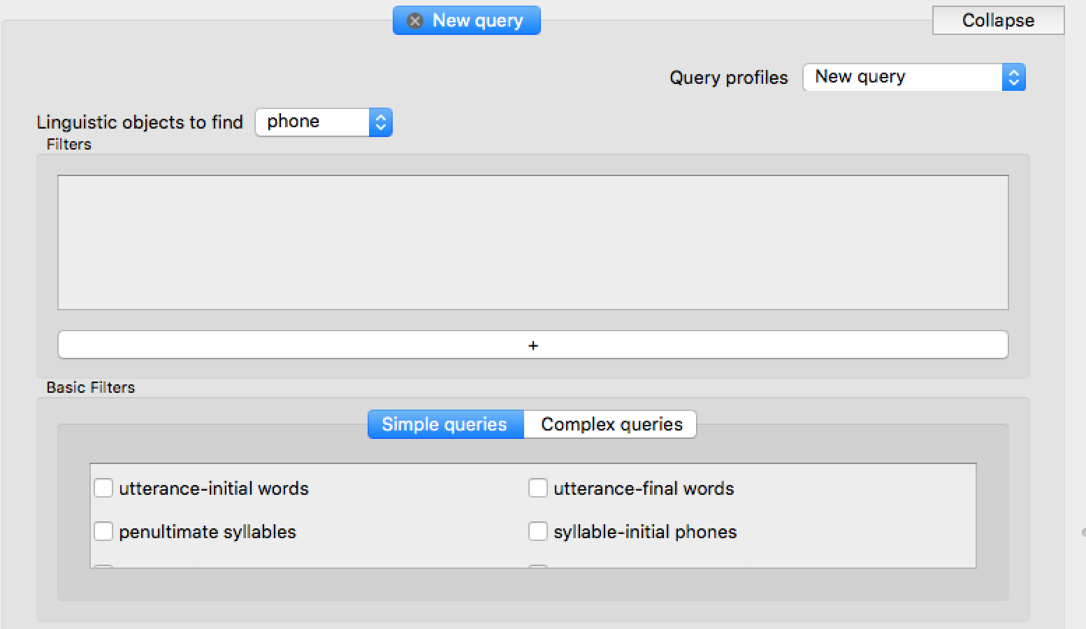
Add filters to the query. A single filter is added by pressing “+” and constructing it, by making selections from drop-down menus which appear. For more information on filters and the intuition behind them, see here.
The first three filters are:
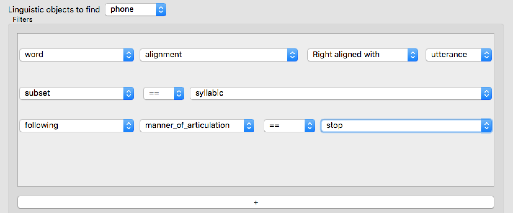
These do the following:
Restrict to utterance-final words :
word: the word containing the phonealignment: something about the word’s alignment with respect to a higher unitRight aligned with,utterance: the word should be right-aligned with its containing utterance
Restrict to syllabic phones (vowels and syllabic consonants):
subset: refer to a “phone subset”, which has been previously defined. Those available in this example includesyllabicsandconsonants.==,syllabic: this phone should be a syllabic.
Restrict to phones followed by a stop (i.e., not a syllabic)
following: refer to the following phonemanner_of_articulation: refer to a property of phones, which has been previously defined. Those available here include “manner_of_articulation” and “place_of_articulation”==,stop: the following phone should be a stop.
Then, add three more filters:
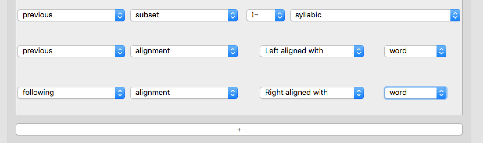
These do the following:
Restrict to phones preceded by a consonant
Restrict to phones which are the second phone in a word
previous: refer to the preceding phonealignment,left aligned with,word: the preceding phone should be left-aligned with (= begin at the same time as) the word containing the target phone. (So in this case, this ensures both that V is preceded by a word-initial C in the same word: #CV.)
Restrict to phones which precede a word-final phone
These filters together form a query corresponding to the desired set of linguistic objects (vowels in utterance-final CVC words, where C2 is a stop).
You should now:
- Save the query : Selecting
Save query profile, and entering a name, such as “LibriSpeech CVC”. - Run the query : Select “Run query”.
Step 2: Creating an export profile
The next step is to export information about each vowel token as a CSV file. We would like the vowel’s duration and identity, as well as the following factors which are expected to affect the vowel’s duration:
- Voicing of the following consonant
- The word’s frequency and neighborhood density
- The utterance’s speech rate
In addition, we want some identifying information (to debug, and potentially for building statistical models):
- What speaker each token is from
- The time where the token occurs in the file
- The orthography of the word.
Each of these 9 variables we would like to export corresponds to one row in an export profile.
To create a new export profile:
Select “New export profile” from the “Export query results” menu.
- Add one row per variable to be exported, as follows: [1]
- Press “+” (create a new row)
- Make selections from drop-down menus to describe the variable.
- Put the name of the variable in the Output name field. (This will be the name of the corresponding column in the exported CSV. You can use whatever name makes sense to you.)
The nine rows to be added for the variables above result in the following export profile:
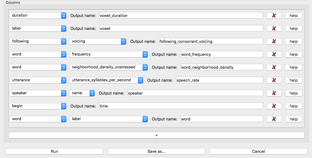
Some explanation of these rows, for a single token: (We use the [u] in /but/ as a running example)
- Rows 1, 2, 8 are the
duration,label, and the beginning time (time) of the phone object (the [u]), in the containing file. - Row 3 refers to the
voicingof the following phone object(the [t])- Note that “following” automatically means “following phone”” (i.e.,
phonedoesn’t need to put put after following) because the linguistic objects being found are phones. If the linguistic objects being found were syllabes (as in Example 2 below), “following” would automatically mean “following syllable”.
- Note that “following” automatically means “following phone”” (i.e.,
- Rows 4, 5, and 9 refer to properties of the word which contains the
phone object: its
frequency,neighborhood density, andlabel(= orthography, here “boot”) - Row 6 refers to the utterance which contains the phone: its
speech_rate, defined as syll`ables per second over the utterance. - Row 7 refers to the speaker (their
name) whose speech contains this phone.
Each case can be thought of as a property (shown in teletype) of a linguistic object or organizational unit (shown in italics).
You can now:
- Save the export profile : Select “Save as...”, then enter a name, such as “LibriSpeech CVC export”.
- Perform the export : Select “Run”. You will be prompted to
enter a filename to export to; make sure it ends in
.csv(e.g.librispeechCvc.csv).
Step 3: Examine the data
Here are the first few rows of the resulting data file, in Excel:

We will load the data and do basic visualization in R. (Make sure that you have the ggplot2 library.)
First, load the data file:
cvc <- read.csv("librispeechCvc.txt")
Voicing
A plot of the basic voicing effect, by vowel:
ggplot(aes(x=following_consonant_voicing, y=vowel_duration), data=cvc) + geom_boxplot() +
facet_wrap(~vowel, scales = "free_y") + xlab("Consonant voicing") + ylab("Vowel duration (sec)")
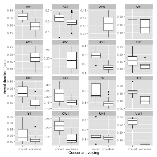
It looks like there is generally an effect in the expected direction, but the size of the effect may differ by vowel.
Speech rate
A plot of the basic speech rate effect, divided up by consonant voicing:
ggplot(aes(x=speech_rate, y=vowel_duration), data=cvc) +
 geom_smooth(aes(color=following_consonant_voicing)) +
geom_point(aes(color=following_consonant_voicing), alpha=0.1, size=1) +
 xlab("Speech rate (sylls/sec)") + ylab("Vowel duration")
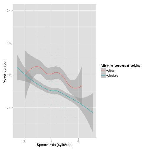
There is a large (and possibly nonlinear) speech rate effect. The size of the voicing effect is small compared to speech rate, and the voicing effect may be modulated by speech rate.
Frequency
A plot of the basic frequency effect, divided up by consonant voicing:
ggplot(aes(x=word_frequency, y=vowel_duration), data=cvc) +
geom_smooth(aes(color=following_consonant_voicing), method="lm") +
geom_point(aes(color=following_consonant_voicing), alpha=0.1, size=1) +
 xlab("Word frequency (log)") + ylab("Vowel duration") + scale_x_log10()
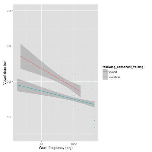
(Note that we have forced a linear trend here, to make the effect clearer given the presence of more tokens for more frequent words. This turns out to be what the “real” effect looks like, once token frequency is accounted for.)
The basic frequency effect is as expected: shorter duration for higher frequency words. The voicing effect is (again) small in comparison, and may be modulated by word frequency: more frequent words (more reduced?) show a smaller effect.
Neighborhood density
In contrast, there is no clear effect of neighborhood density:
ggplot(aes(x=word_neighborhood_density, y=vowel_duration), data=cvc) +
geom_smooth(aes(color=following_consonant_voicing)) +
geom_point(aes(color=following_consonant_voicing), alpha=0.1, size=1) +
xlab("Neighborhood density") + ylab("Vowel duration")
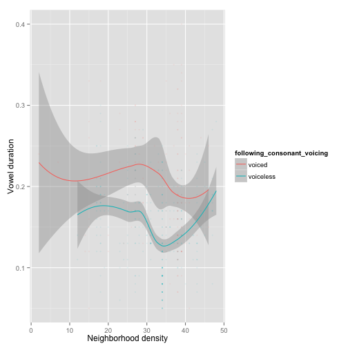
This turns out to be not unexpected, given previous work: while word duration and vowel quality (e.g., centralization) depend on neighborhood density (e.g. Gahl & Yao, 2011), vowel duration has not been consistently found to depend on neighborhood density (e.g. Munson, 2007).
Example 2: Polysyllabic shortening
Motivation
Polysyllabic shortening refers to the “same” rhymic unit (syllable or vowel) becoming shorter as the size of the containing domain (word or prosodic domain) increases. Two classic examples:
- English: stick, sticky, stickiness (Lehiste, 1972)
- French: pâte, pâté, pâtisserie (Grammont, 1914)
Polysyllabic shortening is often – but not always – defined as being restricted to accented syllables. (As in the English, but not the French example.) Using SCT, we can check whether a couple simple versions of polysyllabic shortening holds in the LibriSpeech corpus:
- Considering all utterance-final words, does the initial syllable duration decrease as word length increases?
- Considering just utterance-final words with primary stress on the initial syllable, does the initial syllable duration decrease as word length increases?
We show (1) here, and leave (2) as an exercise.
Step 1: Query profile
In this case, we want to make a query for:
- Word-initial syllables
- ...only in words at the end of utterances (fixed prosodic position)
For this query profile:
“Linguistic objects to find” = “syllables”
- Filters are needed to restrict to:
- Word-initial syllables
- Utterance-final words
This corresponds to the following query profile, which has been saved (in this screenshot) as “PSS: first syllable” in SCT:
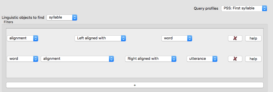
The first and second filters are similar to those in Example 1:
Restrict to word-initial syllables
alignment: something about the syllable’s alignmentleft aligned withword: what it says
Restrict to utterance-final words
word: word containing the syllableright aligned withutterance``: the word and utterance have the same end time.
You should input this query profile, then run it (optionally saving first).
Step 2: Export profile
This query has found all word-initial stressed syllables for words in utterance-final position. We now want to export information about these linguistic objects to a CSV file, for which we again need to construct a query profile. (You should now Start a new export profile.)
We want it to contain everything we need to examine how syllable duration (in seconds) depends on word length (which could be defined in several ways):
- The duration of the syllable
- Various word duration measures: the number of syllables and number of phones in the word containing the syllable, as well as the duration (in seconds) of the word.
We also export other information which may be useful (as in Example 1): the syllable label, the speaker name, the time the token occurs in the file, the word label (its orthography), and the word’s stress pattern.
The following export profile contains these nine variables:

After you enter these rows in the export profile, run the export (optionally saving the export profile first). I exported it as librispeechCvc.csv.
Step 3: Examine the data
In R: load in the data:
pss <- read.csv("librispeechCvc.csv")
There are very few words with 6+ syllables:
library(dplyr)
group_by(pss, word_num_syllables) %>% summarise(n_distinct(word))
## Source: local data frame [6 x 2]
##
##   word_num_syllables n_distinct(word)
##                (int)            (int)
## 1                  1             1019
## 2                  2             1165
## 3                  3              612
## 4                  4              240
## 5                  5               60
## 6                  6                7
So let’s just exclude words with 6+ syllables:
pss <- subset(pss, word_num_syllables<6)
Plot of the duration of the initial stressed syllable as a function of word duration (in syllables):
library(ggplot2)
ggplot(aes(x=factor(word_num_syllables), y=syllable_duration), data=pss) +
geom_boxplot() + xlab("Number of syllables in word") +
ylab("Duration of initial syllable (stressed)") + scale_y_sqrt()
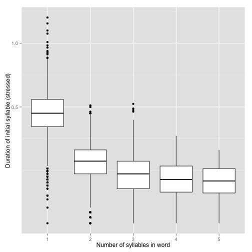
Here we see a clear polysyllabic shortening effect from 1 to 2 syllables, and possibly one from 2 to 3 and 3 to 4 syllables.
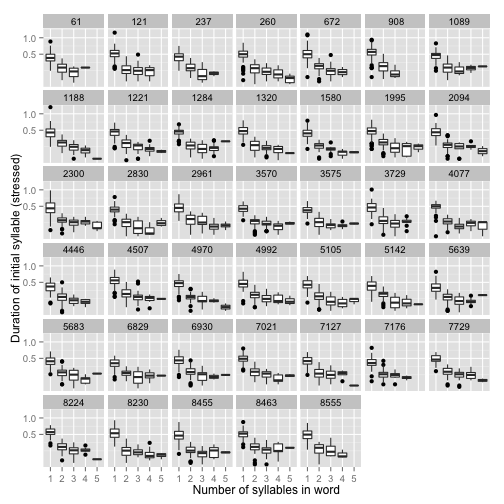
This plot suggests that the effect is pretty robust across speakers (at least for 1–3 syllables):
ggplot(aes(x=factor(word_num_syllables), y=syllable_duration), data=pss) +
geom_boxplot() + xlab("Number of syllables in word") +
ylab("Duration of initial syllable (stressed)") + scale_y_sqrt() + facet_wrap(~speaker)
Example 3: Menzerath’s Law
Motivation: Menzerath’s Law (Menzerath 1928, 1954) refers to the general finding that segments and syllables are shorter in longer words, both in terms of
- duration per unit
- number of units (i.e. segments per syllable)
(Menzerath’s Law is related to polysyllabic shortening, but not the same.)
For example, Menzerath’s Law predicts that for English:
- The average duration of syllables in a word (in seconds) should decrease as the number of syllables in the word increases.
- `` `` for segments in a word.
- The average number of phones per syllable in a word should decrease as the number of syllables in the word increases.
Exercise: Build a query profile and export profile to export a data file which lets you test Menzerath’s law for the LibriSpeech corpus. For example, for prediction (1), you could:
- Find all utterance-final words (to hold prosodic position somewhat constant)
- Export word duration (seconds), number of syllables, anything else necessary.
(This exercise should be possible using pieces covered in Examples 1 and 2, or minor extensions.)
| [1] | Note that it is also possible to input some of these rows automatically, using the checkboxes in the Simple exports tab. |
| [2] | Technically, this database consists of two sub-databases: a Neo4j database (which contains the hierarchical representation of discourses), and a SQL database (which contains lexical and featural information, and cached acoustic measurements). |